Dissecting the Camera Matrix, Part 3: The Intrinsic Matrix
Today we'll study the intrinsic camera matrix in our third and final chapter in the trilogy "Dissecting the Camera Matrix." In the first article, we learned how to split the full camera matrix into the intrinsic and extrinsic matrices and how to properly handle ambiguities that arise in that process. The second article examined the extrinsic matrix in greater detail, looking into several different interpretations of its 3D rotations and translations. Today we'll give the same treatment to the intrinsic matrix, examining two equivalent interpretations: as a description of the virtual camera's geometry and as a sequence of simple 2D transformations. Afterward, you'll see an interactive demo illustrating both interpretations.
If you're not interested in delving into the theory and just want to use your intrinsic matrix with OpenGL, check out the articles Calibrated Cameras in OpenGL without glFrustum and Calibrated Cameras and gluPerspective.
All of these articles are part of the series "The Perspective Camera, an Interactive Tour." To read the other entries in the series, head over to the table of contents.
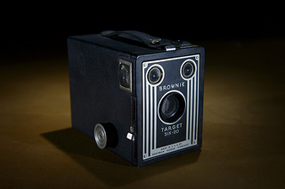
The Pinhole Camera
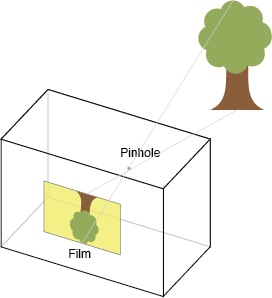
The intrinsic matrix transforms 3D camera cooordinates to 2D homogeneous image coordinates. This perspective projection is modeled by the ideal pinhole camera, illustrated below.
The intrinsic matrix is parameterized by Hartley and Zisserman as
Each intrinsic parameter describes a geometric property of the camera. Let's examine each of these properties in detail.
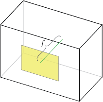
Focal Length, \(f_x\), \(f_y\)
The focal length is the distance between the pinhole and the film (a.k.a. image plane). For reasons we'll discuss later, the focal length is measured in pixels. In a true pinhole camera, both \(f_x\) and \(f_y\) have the same value, which is illustrated as \(f\) below.
In practice, \(f_x\) and \(f_y\) can differ for a number of reasons:
- Flaws in the digital camera sensor.
- The image has been non-uniformly scaled in post-processing.
- The camera's lens introduces unintentional distortion.
- The camera uses an anamorphic format, where the lens compresses a widescreen scene into a standard-sized sensor.
- Errors in camera calibration.
In all of these cases, the resulting image has non-square pixels.
Having two different focal lengths isn't terribly intuitive, so some texts (e.g. Forsyth and Ponce) use a single focal length and an "aspect ratio" that describes the amount of deviation from a perfectly square pixel. Such a parameterization nicely separates the camera geometry (i.e. focal length) from distortion (aspect ratio).
Principal Point Offset, \(x_0\), \(y_0\)
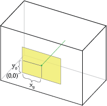
The camera's "principal axis" is the line perpendicular to the image plane that passes through the pinhole. Its itersection with the image plane is referred to as the "principal point," illustrated below.
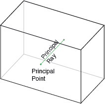
The "principal point offset" is the location of the principal point relative to the film's origin. The exact definition depends on which convention is used for the location of the origin; the illustration below assumes it's at the bottom-left of the film.
Increasing \(x_0\) shifts the pinhole to the right:
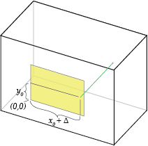
This is equivalent to shifting the film to the left and leaving the pinhole unchanged.
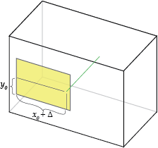
Notice that the box surrounding the camera is irrelevant, only the pinhole's position relative to the film matters.
Axis Skew, \(s\)
Axis skew causes shear distortion in the projected image. As far as I know, there isn't any analogue to axis skew a true pinhole camera, but apparently some digitization processes can cause nonzero skew. We'll examine skew more later.
Other Geometric Properties
The focal length and principal point offset amount to simple translations of the film relative to the pinhole. There must be other ways to transform the camera, right? What about rotating or scaling the film?
Rotating the film around the pinhole is equivalent to rotating the camera itself, which is handled by the extrinsic matrix. Rotating the film around any other fixed point \(x\) is equivalent to rotating around the pinhole \(P\), then translating by \((x-P)\).
What about scaling? It should be obvious that doubling all camera dimensions (film size and focal length) has no effect on the captured scene. If instead, you double the film size and not the focal length, it is equivalent to doubling both (a no-op) and then halving the focal length. Thus, representing the film's scale explicitly would be redundant; it is captured by the focal length.
Focal Length - From Pixels to World Units
This discussion of camera-scaling shows that there are an infinite number of pinhole cameras that produce the same image. The intrinsic matrix is only concerned with the relationship between camera coordinates and image coordinates, so the absolute camera dimensions are irrelevant. Using pixel units for focal length and principal point offset allows us to represent the relative dimensions of the camera, namely, the film's position relative to its size in pixels.
Another way to say this is that the intrinsic camera transformation is invariant to uniform scaling of the camera geometry. By representing dimensions in pixel units, we naturally capture this invariance.
You can use similar triangles to convert pixel units to world units (e.g. mm) if you know at least one camera dimension in world units. For example, if you know the camera's film (or digital sensor) has a width \(W\) in millimiters, and the image width in pixels is \(w\), you can convert the focal length \(f_x\) to world units using:
Other parameters \(f_y\), \(x_0\), and \(y_0\) can be converted to their world-unit counterparts \(F_y\), \(X_0\), and \(Y_0\) using similar equations:
The Camera Frustum - A Pinhole Camera Made Simple
As we discussed earlier, only the arrangement of the pinhole and the film matter, so the physical box surrounding the camera is irrelevant. For this reason, many discussion of camera geometry use a simpler visual representation: the camera frustum.
The camera's viewable region is pyramid shaped, and is sometimes called the "visibility cone." Lets add some 3D spheres to our scene and show how they fall within the visibility cone and create an image.
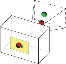
Since the camera's "box" is irrelevant, let's remove it. Also, note that the film's image depicts a mirrored version of reality. To fix this, we'll use a "virtual image" instead of the film itself. The virtual image has the same properties as the film image, but unlike the true image, the virtual image appears in front of the camera, and the projected image is unflipped.
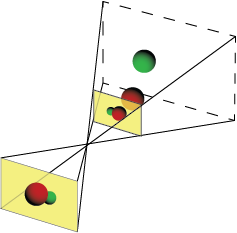
Note that the position and size of the virtual image plane is arbitrary — we could have doubled its size as long as we also doubled its distance from the pinhole.
After removing the true image we're left with the "viewing frustum" representation of our pinhole camera.
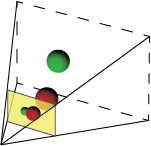
The pinhole has been replaced by the tip of the visibility cone, and the film is now represented by the virtual image plane. We'll use this representation for our demo later.
Intrinsic parameters as 2D transformations
In the previous sections, we interpreted our incoming 3-vectors as 3D image coordinates, which are transformed to homogeneous 2D image coordinates. Alternatively, we can interpret these 3-vectors as 2D homogeneous coordinates which are transformed to a new set of 2D points. This gives us a new view of the intrinsic matrix: a sequence of 2D affine transformations.
We can decompose the intrinsic matrix into a sequence of shear, scaling, and translation transformations, corresponding to axis skew, focal length, and principal point offset, respectively:
An equivalent decomposition places shear after scaling:
This interpretation nicely separates the extrinsic and intrinsic parameters into the realms of 3D and 2D, respactively. It also emphasizes that the intrinsic camera transformation occurs post-projection. One notable result of this is that intrinsic parameters cannot affect visibility — occluded objects cannot be revealed by simple 2D transformations in image space.
Demo
The demo below illustrates both interpretations of the intrinsic matrix. On the left is the "camera-geometry" interpretation. Notice how the pinhole moves relative to the image plane as \(x_0\) and \(y_0\) are adjusted.
On the right is the "2D transformation" interpretation. Notice how changing focal length results causes the projected image to be scaled and changing principal point results in pure translation.
Dissecting the Camera Matrix, A Summary
Over the course of this series of articles we've seen how to decompose
- the full camera matrix into intrinsic and extrinsic matrices,
- the extrinsic matrix into 3D rotation followed by translation, and
- the intrinsic matrix into three basic 2D transformations.
We summarize this full decomposition below.
To see all of these transformations in action, head over to my Perpective Camera Toy page for an interactive demo of the full perspective camera.
Do you have other ways of interpreting the intrinsic camera matrix? Leave a comment or drop me a line!
Next time, we'll show how to prepare your calibrated camera to generate stereo image pairs. See you then!
Posted by Kyle Simek